Trimming Spaces and Merging Columns on Data Sheet
Sometimes you’ll get data sheets that have leading blank spaces in front of the contents of a box. These extra spaces will often mess up the style on your site and throw things out of whack, or even drop the item completely from being imported on your site. You might also want to merge different fields into one.
1. To remove leading white spaces: This process is also covered in the “Using the Filter to Check Info” tutorial, but we’ll go over it here as well. The trim function is used to get rid of leading white spaces.
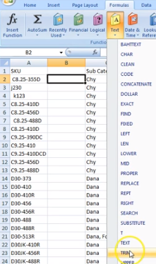
2. The first thing to do is to insert a new column next to the one you’re looking to trim. Something to note, is you’ll never need to work on the top line. The header line isn’t data itself so there’s no need to worry about it until you get to the mapping. Click box 2 of your new column, and in the toolbar, go through “Formulas” -> “Text” -> “TRIM”.
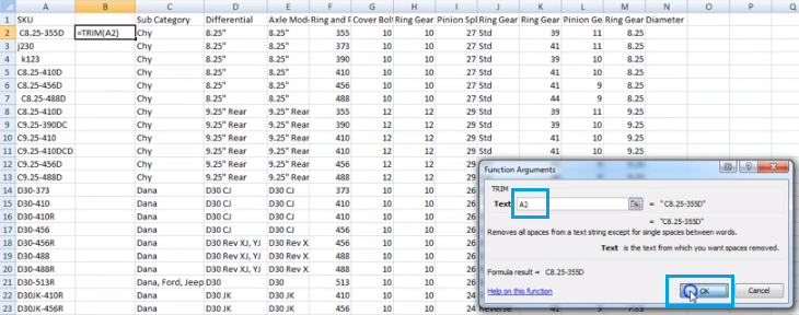
You’ll then see a popup called “Function Arguments”. The Text field is asking for which cell the formula is targeting. Now you’ll need the address of the box you’re applying the formula to. So for example, like in these images if your formul box is B2, the Text field should be A2. Then click “OK”.
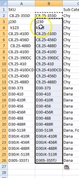
3. Now what you need to do is copy/paste that formula into the rest of the boxes of your new column. Copy the box with the formula, then highlight the rest of the column up to the last row or your data sheet, and paste. One quick way of highlighting all the values without dragging your mouse to the bottom would be: copy the formula box, scroll to the last value of the data sheet, while holding the shift key down click on the last empty box in your new column that would hold a data value.
4. There is one last step for the trimming portion. Only the formulas will be read and mess up your import if you were to keep the formula column as is. So this next step is imperative to make sure the importer reads the actual value, and not the formula.
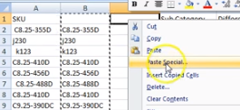
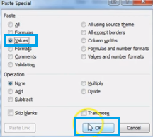
5. You’ll now want to insert a new column, copy the column with the formula, and “Paste Special” into the header box of the newest column. In the popup, change the Paste selection to “Values” and click “OK”.
6. You’ll then notice in the newest column, it contains the value instead of the formula. You can now copy/paste the column header into the newest column, and delete the original and the one with the formula.
7. To Merge Columns/Concatenation: If you ever want to merge two different columns into one, like for example if you want to amend a column and add one to the description, that’s done through concatenation.
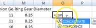
8. For this as well, you can ignore the header bar. In the second box of a new column, you’ll want to type “=concatenate”, and double-click on the all caps concatenate option that comes up.
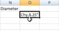
9. Next it will ask you for the addresses of the boxes you’re looking to combine. Click on the first box you want, then add a comma and within a pair of quotation marks specify how you want these two pieces of information seperated. By default, Excel will merge these values with no spaces or anything in between, so if you want a space, a comma, an ampersand, etc., add it between the quotation marks. After the quotation marks you’ll need to add another comma. Then you can click on the second box you want to add. Once you’ve added all the boxes you’d like to concatenate, close the parentheses and hit your enter key. Here’s an example of what it will look like:

10. Now you can repeat steps 3-5 of copy/pasting this formula into the rest of the column, then type the new header for that field! :)