Using the Filter to Check Data Sheet Info
These instructions should help speed up your importing process by cleaning up CSV sheets to import neatly. This covers how to search for duplicate values, missing/blank fields, trimming data to get rid of leading spaces, and more.
1. A good general tip for when you’re working on these spreadsheets is to adjust the row height to keep the rows from becoming overstretched and taking up screen room. You can do this by selecting the whole sheet in the upper left-hand corner of the sheet, right click anywhere in the space -> “Row Height”, type 15 and click ok.
2. To find out if there are duplicates:
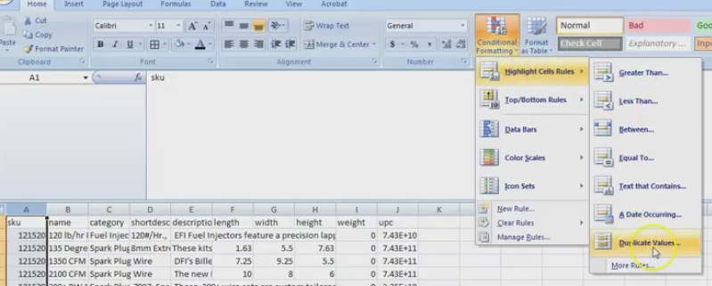
a. Highlight the column by selecting the column letter, then in the toolbar select “Conditional Formatting” -> “Highlight Cells Rules” -> “Duplicate Values”
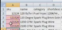
The column will now highlight the elements with duplicate values in that column. A pop up titled “Duplicate Values” will let you select the color you want, then click ok. Once the value is changed, and it is not a duplicate, the highlight will clear itself out for the changed box like so:
Or if you need to undo all the highlights for any reason, go to “Conditional Formatting”
-> “Clear Rules” and select which you would like to clear.
Duplicate values are usually in the SKU and title/name columns and sometimes in the UPC column, so those are always a good idea to check. There’s no need to check the description or price columns.
3. Checking for blank or invalid fields such as no category, no pricing, no shipping details, no images, etc.:
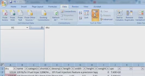
a. In the toolbar, go to “Data” -> “Filter” and you’ll see dropdown arrows pop up next to the title for each of your columns.
Click on that dropdown arrow, and you’ll see a shorthand list of all the entries in this column. This is a good way to check invalid entries, like words in a number pricing column, etc. If you scroll to the bottom of the list, you’ll see an entry titles “Blanks”
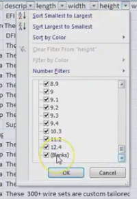
If you see this, scroll back to the top, and deselect “Select all” at the top of this list, then scroll back down to the bottom and select “Blanks”, then “Ok”. You’ll then see a change in the excel sheet because it’s narrowed down to only display the blank items for that column. You can then make the necessary corrections and watch the items disappear once their corrected. If you want to see all the items again, go back through the dropdown arrow and check the “Select all” box.
Checking Category Names: Categories are tricky, since you’re getting data from different sources and they all have their own naming conventions. If you scroll through the categories dropdown list, you’ll be able to see if there is a variation of a category that does not match to one on yours. For example, if there is a category on the data sheet for “Fuel Pumps”, but the corresponding category on your site is “Fuel Pump”, you will want to use the filter to select only items under “Fuel Pumps” and remove that last letter. If this is not done, an extra category will be added to your site, and you’ll end up with two different fuel pump categories. Don’t forget to check for blank categories as well.
b. Checking for spaces in short descriptions: It’s always a safe bet to eliminate any existing spaces in front of the short descriptions. If there are any leading spaces, it could cause issues with the styling on your site or issues with any bots.
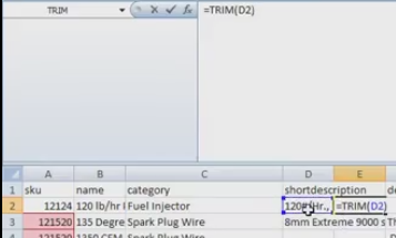
i. First thing is to create or go to a new blank column. In the new column, row 2, type in the trim formula for the first short description. You can either type the address of the corresponding short description block within the parentheses, or when you get there just click on the bock (=TRIM(D2))
Once the formula is typed in, hit he enter key, copy the box with the formula, and highlight the rest of the boxes in that new column, all the way down to the last item. Then paste the formula in those boxes.
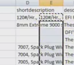
At this point, you’ll be able to visibly notice in the new row, all the information is lined up at the start of the column.
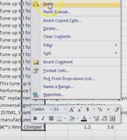
ii. At this point, highlight the entire new column and copy it. Then in the first cell of the old description column, “Paste Special” the column you just copied:
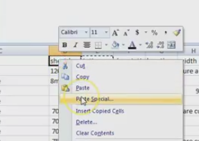
This way, the values instead of the formula are pasted over.
iii. You can them delete the column used for the formulas, and in the first cell of the newly trimmed values that were just pasted in, you’ll need to put your header back in there.