Working with Filter and Proper Capitalization on Excel
Here we’ll go over how to change all caps on your data sheet into proper format of the first letter of each word capitalized, and how to use the filter to edit information. You want to make sure your data is not in all uppercase, because the all caps will cause problems.
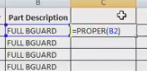
1. There’s a formula you can use to get rid of all caps. The first thing you’ll need to do is insert a new column next to whichever column you want to remove the all uppercase from. In the second box in your new blank column (you do not need to convert the header row), start typing “=proper”, once it comes up as one of the options, double-click it, then click the cell to the left that box so it grabs its address. You can then close the parentheses, and hit enter on your keyboard. It should end up looking something like this before you click enter, then the next photo after:
2. Now it’s time to copy/paste that formula in the rest of the boxes in your new column. Click the one box with the formula, and copy it, then scroll to the bottom of the data sheet and while holding down the shift key on your keyboard, click the last box in that column that will hold a value. Right click and select paste.
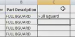
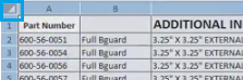
3. You should now see the contents of your new column (except the first box) will mimic the column before it, except with only the first letter of each word capitalized.
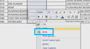
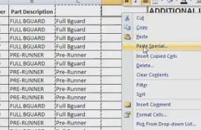
4. Now you’ll want to copy/paste the values from your new column into another one. This step is imperative because your importer will not understand the formula itself, so you’ll need to convert it to the text that you see. Highlight the newly formulated column and copy it, then next to it highlight a new and blank column, right click, and select “Paste Special”. In the popup, under paste, select “Values”, then “OK”. This way, the new values are pasted, and not the formulas.
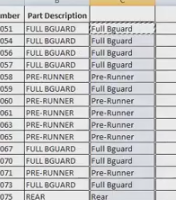
5. Now you can copy/paste the original column title, or just rename it, and delete the original column, and the column with the formula. This way only the new valued column is in place for that field.
6. To use the filter: The filter can be used to take care of any blank fields, unwanted items, misnamed items, etc.
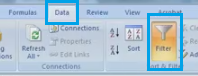
7. To apply the filter, click on the box to the top left corner of your sheet between the A1 column/row marker, which will highlight your whole sheet, then from the toolbar select “Data” -> “Filter”.
8. You’ll then see the header to each column will have a dropdown arrow that lists all the contents of that column. You can use this to go through and select for only the improper values to show so that you can correct them. You can go column by column to correct any values. There are mor extensive examples on using the filter in another tutorial called “Using the Filter to Check Info”.